24:20
Ch4-13 t test
Statistics NYCU
Overview
This video explains how to perform hypothesis tests and construct confidence intervals for population means using small sample sizes (less than 30). It introduces the t-test as an alternative to the z-test when the population standard deviation is unknown and the sample size is small. The video details the assumptions for the t-test (normal population distribution), the calculation of the t-statistic, the concept of degrees of freedom, and how to interpret the results using critical values or p-values, contrasting it with the z-test and illustrating with two practical examples.
How was this?
Save this permanently with flashcards, quizzes, and AI chat
Chapters
- Inferential statistics uses sample data to make conclusions about a population.
- Estimation involves point estimates (single value) and interval estimates (range with confidence level).
- Hypothesis testing involves setting up null and alternative hypotheses and using sample data to decide whether to reject the null hypothesis.
- The z-test is used for large samples or when population standard deviation is known; the t-test is for small samples with unknown population standard deviation.
Understanding these foundational concepts is crucial for making informed decisions and drawing valid conclusions from data when dealing with uncertainty.
Estimating a population mean using a sample mean and a confidence interval, or testing if a population mean is equal to a specific value (e.g., mu = 50).
- When sample size is small (n < 30) and population standard deviation is unknown, the t-test is used.
- A key assumption for the t-test is that the population from which the sample is drawn is normally distributed.
- The t-statistic is calculated similarly to the z-statistic but uses the sample standard deviation to estimate the population standard deviation.
- The t-distribution is similar to the normal distribution but has heavier tails, meaning it's wider, especially for small sample sizes.
This allows us to perform valid statistical tests and construct reliable confidence intervals even when we have limited data, which is common in many real-world scenarios.
Using sample mean, sample standard deviation, and sample size to calculate a t-statistic for hypothesis testing.
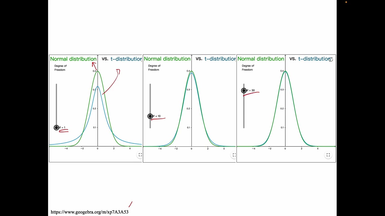
- The t-distribution has a parameter called degrees of freedom (df), typically calculated as n-1.
- As degrees of freedom increase (i.e., as sample size increases), the t-distribution approaches the standard normal (z) distribution.
- For small degrees of freedom, the t-distribution is wider than the z-distribution, reflecting greater uncertainty.
- T-distribution tables provide critical values for specific degrees of freedom and significance levels (alpha).
Understanding degrees of freedom is essential for correctly identifying the appropriate t-distribution curve and finding the correct critical values for hypothesis testing.
Comparing the shape of the t-distribution with df=1, df=10, and df=30 to the z-distribution, showing how it becomes narrower and closer to the z-distribution as df increases.
- Set up the null (H0) and alternative (Ha) hypotheses.
- Determine the significance level (alpha).
- Calculate the t-test statistic using the formula: t = (sample mean - hypothesized mean) / (sample standard deviation / sqrt(sample size)).
- Determine the critical value(s) from the t-distribution table using alpha and degrees of freedom, or calculate the p-value.
- Compare the calculated t-statistic to the critical value(s) or compare the p-value to alpha to make a decision: reject H0 or fail to reject H0.
Following these steps systematically ensures that hypothesis tests are conducted correctly, leading to reliable conclusions about population parameters.
A traffic engineer testing if the average red light duration is significantly different from 60 seconds, using a sample of 36 lights.
- The problem involves testing if the average red light duration is significantly different from 60 seconds (a two-tailed test).
- Sample size (n=36) is large enough that a z-test could be used, but a t-test is demonstrated for learning purposes.
- Hypotheses: H0: μ = 60, Ha: μ ≠ 60. Significance level α = 0.05.
- Calculated t-statistic is 2.25. With df=35, this value falls into the rejection region, leading to the rejection of the null hypothesis.
- Conclusion: There is evidence that the average red light duration is significantly different from 60 seconds.
This example demonstrates how to apply the t-test procedure to a real-world problem and interpret the statistical findings in a practical context.
A traffic engineer claims the average red light duration is 60 seconds. A sample of 36 lights shows a mean of 63 seconds with a standard deviation of 8 seconds. The t-test leads to rejecting the claim.
- The problem tests if the average commuting time is less than 30 minutes (a one-tailed test).
- Sample size (n=20) is small, and the population is assumed to be normally distributed.
- Hypotheses: Ha: μ < 30, H0: μ ≥ 30. Significance level α = 0.05.
- Calculated t-statistic is -2.18. With df=19, this value falls into the rejection region for a left-tailed test.
- Conclusion: There is evidence that the average commuting time is less than 30 minutes.
This example illustrates how to conduct a one-tailed t-test and draw conclusions when the research question is directional (e.g., 'less than' or 'greater than').
A company wants to know if its employees' average commute time is less than 30 minutes. A sample of 20 employees has a mean commute of 28 minutes and a standard deviation of 5 minutes. The t-test supports the claim that it's less than 30 minutes.
Key takeaways
- The t-test is essential for hypothesis testing and confidence intervals with small sample sizes when the population standard deviation is unknown.
- The assumption of a normally distributed population is critical for the validity of the t-test, especially with very small sample sizes.
- Degrees of freedom (n-1) adjust the t-distribution based on sample size, making it wider for smaller samples and approaching the z-distribution for larger samples.
- Hypothesis testing decisions are made by comparing a calculated test statistic (t-value) to a critical value or by comparing the p-value to the significance level (alpha).
- The choice between a one-tailed and two-tailed test depends on the specific research question or claim being investigated.
- Statistical software can provide exact p-values and critical values, while tables often provide ranges, requiring estimation.
- Interpreting the results requires stating a conclusion in the context of the original problem, not just stating whether the null hypothesis was rejected.
Key terms
T-testSmall samplePopulation standard deviationSample standard deviationT-distributionDegrees of freedom (df)Hypothesis testingNull hypothesis (H0)Alternative hypothesis (Ha)Significance level (alpha)Critical valueP-valueOne-tailed testTwo-tailed test
Test your understanding
- Why is the t-test necessary when dealing with small sample sizes and an unknown population standard deviation?
- How does the t-distribution differ from the z-distribution, and how does the degree of freedom influence this difference?
- What are the key assumptions that must be met to perform a valid t-test for a population mean?
- Describe the process of conducting a two-tailed t-test, including setting hypotheses, calculating the test statistic, and making a decision.
- How would you determine whether to use a one-tailed or two-tailed t-test based on a given research question?