AI-Generated Video Summary by NoteTube
Markov Chains Clearly Explained! Part - 1
Normalized Nerd
Overview
This video introduces the concept of Markov chains, explaining their fundamental properties and applications. It uses a restaurant example serving hamburgers, pizza, and hot dogs, where the next day's food depends only on the current day's offering. The video defines states, transitions, and the crucial Markov property: the future depends solely on the present, not the past. It illustrates how to calculate probabilities and introduces the idea of a "random walk" through the chain. The concept of a stationary distribution, where probabilities stabilize over time, is explored through simulation and then explained more rigorously using linear algebra and the transition matrix. The video concludes by showing how to find the stationary distribution by solving for the left eigenvector with an eigenvalue of 1, relating it to concepts from linear algebra.
This summary expires in 30 days. Save it permanently with flashcards, quizzes & AI chat.
Chapters
- •Markov chains are used across various fields like statistics, biology, economics, physics, and machine learning.
- •The video aims to provide a clear understanding of Markov chains and their significance.
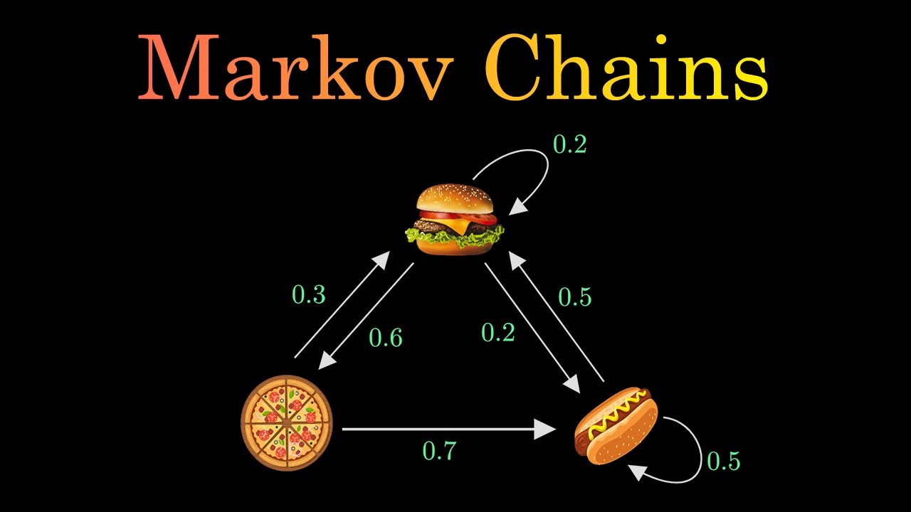
- •A restaurant example is introduced: serving hamburgers, pizza, or hot dogs.
- •The choice of food for a given day depends only on the previous day's choice.
- •Each food item (hamburger, pizza, hot dog) represents a 'state'.
- •The probability of moving from one state to another is called a 'transition'.
- •These transitions can be visualized as weighted arrows in a diagram.
- •A diagram showing all possible transitions is a Markov chain.
- •The core property: the future state depends only on the current state, not on the sequence of events that preceded it.
- •Mathematically: P(X_n+1 | X_n, X_n-1, ..., X_0) = P(X_n+1 | X_n).
- •This property simplifies complex real-world problems.
- •Example: Probability of serving hot dogs tomorrow only depends on today's food, not yesterday's or the day before.
- •The sum of probabilities of outgoing transitions from any state must equal 1.
- •This ensures that probabilities are valid and cover all possibilities.
- •The video focuses on basic Markov chains, acknowledging special types exist.
- •A 'random walk' simulates moving through the states over time.
- •After many steps, the distribution of states can be calculated (e.g., % of days serving each food).
- •The probabilities tend to converge to fixed values over a large number of steps.
- •This stable probability distribution is called the 'stationary distribution' or 'equilibrium state'.
- •Markov chains can be represented by a 'transition matrix' (adjacency matrix with probabilities).
- •A 'row vector' (pi) represents the probability distribution of states.
- •Multiplying the current state vector by the transition matrix yields the next state vector.
- •The stationary state (pi) satisfies the equation: pi * A = pi, where A is the transition matrix.
- •The equation pi * A = pi is related to finding eigenvectors.
- •Specifically, pi is the left eigenvector of A with an eigenvalue of 1.
- •The elements of pi must sum to 1 (probability distribution constraint).
- •Solving these two conditions yields the stationary distribution.
- •This method allows checking for multiple stationary states (multiple eigenvectors with eigenvalue 1).
Key Takeaways
- 1Markov chains model systems where future states depend only on the current state.
- 2The Markov property (memorylessness) is fundamental to simplifying complex systems.
- 3Transitions between states are defined by probabilities.
- 4A random walk simulates movement through states, and probabilities can converge over time.
- 5The stationary distribution represents the long-term probability of being in each state.
- 6Linear algebra, particularly transition matrices and eigenvectors, provides a powerful tool to calculate stationary distributions.
- 7The equation pi * A = pi, where pi is the state vector and A is the transition matrix, is key to finding the stationary state.
- 8The stationary distribution is the left eigenvector of the transition matrix corresponding to the eigenvalue 1, with elements summing to 1.